Simulate particles and write STAR file
%load_ext autoreload
%autoreload 2
This tutorial demonstrates how to simulate a cryo-EM dataset through cryoJAX's built-in STAR file utilities. In doing so, the tutorial builds off of the tutorial demonstrating how to make custom image simulation methods.
This tutorial is split into three parts:
1) Generate a STAR file of particle parameters
2) Define an image simulator given those parameters and a custom AbstractVolumeParametrization
3) Simulate images with added noise and write to the STAR file and to disk.
This process is designed to be flexible: users design their own image formation model to generate a dataset. This tutorial can easily be adapted or modified to include additional functionality.
# Plotting imports and functions
from matplotlib import pyplot as plt
from mpl_toolkits.axes_grid1 import make_axes_locatable


def plot_image(image, fig, ax, cmap="gray", label=None, **kwargs):
    im = ax.imshow(image, cmap=cmap, origin="lower", **kwargs)
    divider = make_axes_locatable(ax)
    cax = divider.append_axes("right", size="5%", pad=0.05)
    fig.colorbar(im, cax=cax)
    if label is not None:
        ax.set(title=label)
    return fig, ax
To start, generate particle parameters and write a STAR file.
To do this, first we must vmap over JAX random number generator keys and sample particle parameters for the pose and CTF. You can adapt this function to your needs, such as adapting the range of the distributions for the random parameters, or changing wheter a parameter is random or not.
Then, save a STAR file using the utilities in the cryojax.dataset submodule.
import cryojax.simulator as cxs
import equinox as eqx
import jax
import jax.numpy as jnp
from cryojax.rotations import SO3
from jaxtyping import PRNGKeyArray


@eqx.filter_vmap(in_axes=(0, None))
def make_particle_parameters(key: PRNGKeyArray, config: cxs.BasicImageConfig):
    """Generate random parameters."""
    # Pose
    # ... instantiate rotations
    key, subkey = jax.random.split(key)  # split the key to use for the next random number
    rotation = SO3.sample_uniform(subkey)

    # ... now in-plane translation
    ny, nx = config.shape

    key, subkey = jax.random.split(key)  # do this everytime you use a key!!
    offset_in_angstroms = (
        jax.random.uniform(subkey, (2,), minval=-0.1, maxval=0.1)
        * jnp.asarray((nx, ny))
        / 2
        * config.pixel_size
    )
    # ... build the pose
    pose = cxs.EulerAnglePose.from_rotation_and_translation(rotation, offset_in_angstroms)

    # CTF Parameters
    # ... defocus
    key, subkey = jax.random.split(key)
    defocus_in_angstroms = jax.random.uniform(subkey, (), minval=10000, maxval=15000)
    # ... astigmatism
    key, subkey = jax.random.split(key)
    astigmatism_in_angstroms = jax.random.uniform(subkey, (), minval=0, maxval=100)
    key, subkey = jax.random.split(key)
    astigmatism_angle = jax.random.uniform(subkey, (), minval=0, maxval=jnp.pi)
    # Now non-random values
    spherical_aberration_in_mm = 2.7
    amplitude_contrast_ratio = 0.1
    # Build the CTF
    transfer_theory = cxs.ContrastTransferTheory(
        ctf=cxs.AstigmaticCTF(
            defocus_in_angstroms=defocus_in_angstroms,
            astigmatism_in_angstroms=astigmatism_in_angstroms,
            astigmatism_angle=astigmatism_angle,
            spherical_aberration_in_mm=spherical_aberration_in_mm,
        ),
        amplitude_contrast_ratio=amplitude_contrast_ratio,
    )

    return {
        "image_config": config,
        "pose": pose,
        "transfer_theory": transfer_theory,
    }


# Generate particle parameters. First, the image config

config = cxs.BasicImageConfig(
    shape=(150, 150),
    pixel_size=2.0,
    voltage_in_kilovolts=300.0,
    padded_shape=(200, 200),
)
# ... RNG keys
number_of_images = 100
keys = jax.random.split(jax.random.key(0), number_of_images)
# ... make parameters
particle_parameters = make_particle_parameters(keys, config)
import cryospax as spx


# Generate STAR file
make_image_config = lambda _shape, _pixel_size, _voltage_in_kilovolts: (
    cxs.BasicImageConfig(
        _shape,
        _pixel_size,
        _voltage_in_kilovolts,
        padded_shape=config.padded_shape,
    )
)
parameter_file = spx.RelionParticleParameterFile(
    path_to_starfile="./outputs/particles.star",
    mode="w",  # writing mode!
    max_optics_groups=1,  # maximum allowed optics group writes
    exist_ok=True,  # in case the file already exists
    options=dict(make_image_config=make_image_config),
)
parameter_file.append(particle_parameters)
parameter_file.save(overwrite=True)
Next, create a custom AbstractVolumeParametrization to simulate images randomized over a structure's discrete conformations. We will simulate images of thyroglobulin in two conformations. See the tutorial for creating cryoJAX extensions for more information.
from typing_extensions import override

from jaxtyping import Array, Float, Int


class DiscreteConformationSampler(cxs.AbstractVolumeParametrization):
    """Sample discrete conformational heterogeneity.

    Note that sampling occurs upon intialization and the conformation
    index sampled is stored.
    """

    sampled_volume: cxs.AbstractVolumeRepresentation
    conformation: Int[Array, ""]

    def __init__(
        self,
        rng_key: PRNGKeyArray,
        conformational_space: tuple[cxs.AbstractVolumeRepresentation, ...],
        weights: tuple[float, ...] | Float[Array, " _"],
    ):
        assert len(conformational_space) == len(weights)
        n_conformations = len(conformational_space)
        conformation = jax.random.choice(
            rng_key, jnp.arange(n_conformations), p=jnp.asarray(weights, float)
        )
        # Assumes that the `AbstractVolumeRepresentation` is a pytree
        # of arrays only. Otherwise, calls to `equinox.partition` and
        # `equinox.combine` would be necessary
        stacked_volume = jax.tree.map(
            lambda *xs: jnp.stack(xs, axis=0), *conformational_space
        )
        self.sampled_volume = jax.tree.map(lambda x: x[conformation], stacked_volume)
        self.conformation = conformation

    @override
    def to_representation(
        self, rng_key: PRNGKeyArray | None = None
    ) -> cxs.AbstractVolumeRepresentation:
        return self.sampled_volume


def make_conformational_space(paths_to_pdb: list[str]):
    """Instantiate a `DiscreteConformationSampler`
    simply given multiple paths to PDB files.
    """
    for path_to_pdb in paths_to_pdb:
        yield cxs.load_tabulated_volume(
            path_to_pdb,
            selection_string="name CA",
            include_b_factors=True,
            output_type=cxs.GaussianMixtureVolume,
        )


conformational_space = tuple(
    make_conformational_space(
        ["./data/thyroglobulin_unbent.pdb", "./data/thyroglobulin_bent.pdb"]
    )
)
Now, define a function that simulates images given the DiscreteConformationSampler. Ultimately this will be passed to the cryospax.simulate_particle_stack utility. For reasons we will see, the following function signature is required.
def simulate_fn(particle_parameters, constant_args, per_particle_args):
    """Compute a single image from the given particle parameters.

    **Arguments:**

    - `particle_parameters`:
        A dictionary containing the parameters for the particle.
        This is an element of a `RelionParticleParameterFile`.
    - `constant_args`:
        A PyTree whose arrays do not have a batch dimension, i.e. they stay
        constant across all particles.
    - `per_particle_args`:
        A PyTree whose arrays have a batch dimension matching the number of
        particles in `particle_parameters`.
    """
    ...
In this function, we will simulate images at a randomly sampled SNR.
Simulating images at a given SNR
The GaussianWhiteNoiseModel in cryoJAX simulates images as image = signal + noise.
The signal is normalized by defining a region where we know there is signal, where we can measure the
mean and standard deviation of our simulated image without noise. After normalizing, we can set the signal-to-noise ratio (SNR) by setting the noise variance to 1 and the signal variance equal to the SNR. The latter step is simply done by scaling the normalized image by a constant.
import cryojax.ndimage as im
import jax.random as jr


def simulate_fn(particle_parameters, conformational_space, rng_key):
    # Generate RNG keys for each part of the process
    conformation_rng_key, noise_rng_key, snr_rng_key = jr.split(rng_key, 3)
    # Build image model, including normalization within a circular mask
    # around each particle
    image_config, pose, transfer_theory = (
        particle_parameters["image_config"],
        particle_parameters["pose"],
        particle_parameters["transfer_theory"],
    )
    mask = im.CircularCosineMask(
        coordinate_grid=image_config.get_coordinate_grid(physical=True),
        radius=150.0,
        rolloff_width=0.0,
        xy_offset=pose.offset_in_angstroms,
    )
    volume = DiscreteConformationSampler(
        conformation_rng_key, conformational_space, weights=(0.5, 0.5)
    )
    image_model = cxs.make_image_model(
        volume,
        pose=pose,
        image_config=image_config,
        transfer_theory=transfer_theory,
        normalizes_signal=True,
        signal_region=mask.get() == 1.0,
    )
    # Build noise model at a randomly sampled SNR within a
    # uniform range, then simulate
    snr = jax.random.uniform(snr_rng_key, minval=0.01, maxval=0.1)
    noise_model = cxs.GaussianWhiteNoiseModel(
        image_model,
        variance=1.0,
        signal_scale_factor=jnp.sqrt(snr),
    )

    return noise_model.sample(rng_key=noise_rng_key)


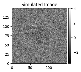
# Simulate a test image
fig, ax = plt.figure(figsize=(3, 3)), plt.gca()
test_parameters = parameter_file[0]
image = simulate_fn(test_parameters, conformational_space, rng_key=jax.random.key(1234))
plot_image(image, fig, ax, label="Simulated Image")
(<Figure size 300x300 with 2 Axes>,
 <Axes: title={'center': 'Simulated Image'}>)
Finally, simulate a dataset using cryospax.simulate_particle_stack.
The simulate_particle_stack tool
This function takes in two key arguments: a STAR file and a function
that simulates images. We just defined the latter, but we also need
build off of the RelionParticleParameterFile we defined and build what
is called a RelionParticleDataset. This specifies how to write
the MRC files.
import pathlib


# Instantiate MRC I/O via the `RelionParticleDataset`
path_to_relion_project = "./outputs/"
mrcfile_output_folder = "images/"
path_to_mrcfiles = pathlib.Path(path_to_relion_project, mrcfile_output_folder)
if not path_to_mrcfiles.exists():
    path_to_mrcfiles.mkdir(parents=True, exist_ok=False)

dataset = spx.RelionParticleDataset(
    parameter_file,
    path_to_relion_project=path_to_relion_project,
    mode="w",
    mrcfile_options={"overwrite": True, "output_folder": mrcfile_output_folder},
)
Finally, let's use simulate_particle_stack to simulate images.
rng_keys = jax.random.split(jax.random.key(seed=1234), num=len(dataset))
spx.simulate_particle_stack(
    dataset,
    simulate_fn,
    constant_args=conformational_space,
    per_particle_args=rng_keys,
    batch_size=None,  # how many images to simulate in parallel
    images_per_file=50,  # how many images in each MRC file
    overwrite=True,
)
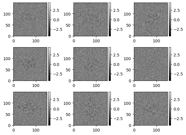
Finally, as we saw in the load cryo-EM images tutorial, we can load images and parameters using the RelionParticleDataset.
import math


def plot_image_stack(images, cmap="gray", **kwargs):
    n_images_per_side = int(math.sqrt(images.shape[0]))
    fig, axes = plt.subplots(nrows=n_images_per_side, ncols=n_images_per_side)
    vmin, vmax = images.min(), images.max()
    for idx, ax in enumerate(axes.ravel()):
        im = ax.imshow(
            images[idx], cmap=cmap, vmin=vmin, vmax=vmax, origin="lower", **kwargs
        )
        divider = make_axes_locatable(ax)
        cax = divider.append_axes("right", size="5%", pad=0.05)
        fig.colorbar(im, cax=cax)
    fig.tight_layout()


particles = dataset[0:9]
plot_image_stack(particles["images"])